Array Data Structure: Memory Layout, Operations and Worked Examples
Understand how arrays map indices to memory, then practise address calculation, exact shift counts, searching and dynamic-array growth with worked examples.
KnowledgeGate Team
Exam prep & CS education
Updated 24 Oct 20266 min read
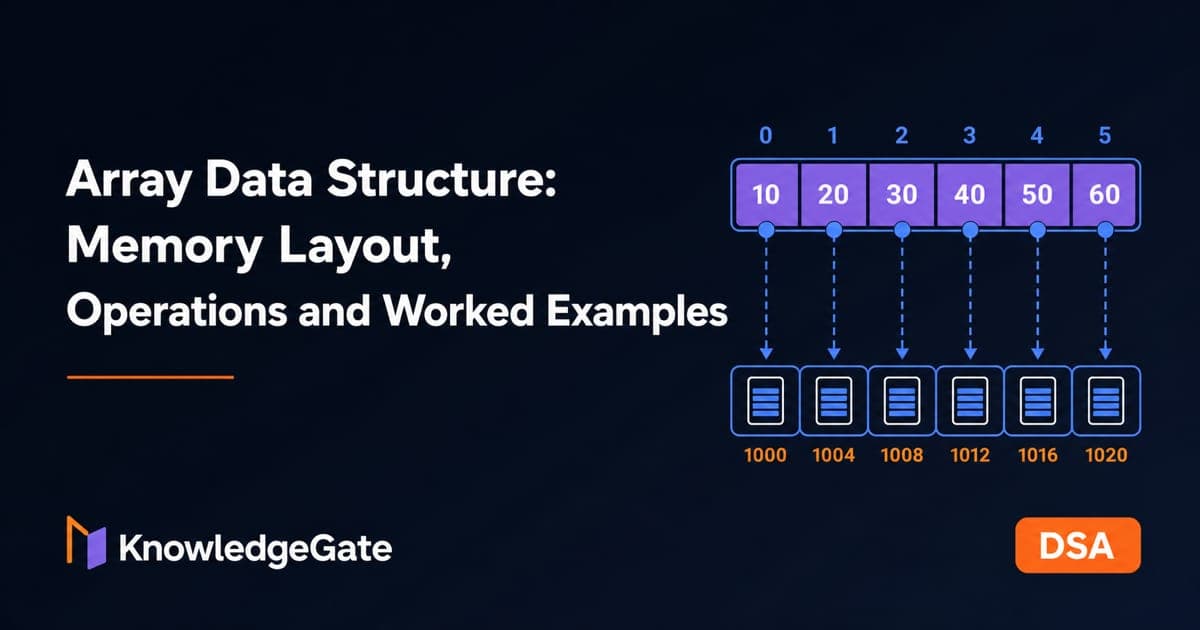
An array looks simple until an address-calculation problem introduces lower bounds, or an insertion question asks for the exact number of shifts. Then an index, a position and an address can start looking like the same thing. Contiguous, same-type storage means that the base address, element width and index bounds determine every offset.
Array data structure: the mental model and core properties
An array is a logical sequence of homogeneous elements stored in contiguous memory. Each position has an index, and a fixed index-to-offset rule maps that index to an address.
Take A = [12, 7, 25, 9, 18, 31], indexed from 0 to 5. Here, A[3] = 9 means index 3, the fourth position, stores value 9. Its address depends on the base address and element width. Index, position, value and address are distinct.
A one-dimensional array is a line. Two-dimensional and higher-dimensional arrays use more indices. A matrix is a programmer's grid, but memory holds one linear run of words in row-major or column-major order.
Separate logical size from capacity. With capacity 8, storage is [12, 7, 25, 9, 18, 31, _, _]. Logical size is 6, occupied indices are 0..5, and indices 6 and 7 are spare slots, not readable elements.
For cross-structure selection, Data Structures: Types, Operations, Complexity, and Worked Examples compares arrays with linked lists under one workload. Array-specific questions add address formulas, exact shifts, search preconditions and resize costs.
Array address calculation: row-major and column-major worked example
For a two-dimensional array with base address B, element width w, row lower bound Lr, column lower bound Lc, Nr rows and Nc columns:
Row-major:
LOC(M[i][j]) = B + w((i-Lr)Nc + (j-Lc))Column-major:
LOC(M[i][j]) = B + w((j-Lc)Nr + (i-Lr))
Row-major counts complete rows of Nc elements, then preceding elements in the target row. Column-major counts complete columns of Nr elements, then preceding elements in the target column.
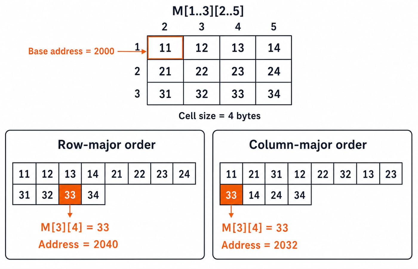
Consider M[1..3][2..5], a 3 x 4 integer array:
Row | Values |
|---|---|
1 | 11, 12, 13, 14 |
2 | 21, 22, 23, 24 |
3 | 31, 32, 33, 34 |
Let B = LOC(M[1][2]) = 2000 and w = 4 bytes. Find the address of M[3][4] = 33.
In row-major order, two complete rows and two more elements come first:
((3-1) x 4 + (4-2)) x 4 = (8 + 2) x 4 = 40 bytes.
Therefore, LOC(M[3][4]) = 2000 + 40 = 2040.
In column-major order, two complete columns and two more elements come first:
((4-2) x 3 + (3-1)) x 4 = (6 + 2) x 4 = 32 bytes.
Therefore, LOC(M[3][4]) = 2000 + 32 = 2032.
For a zero-based integer array at base 1000, the one-dimensional check is LOC(A[3]) = 1000 + (3-0) x 4 = 1012.
Array insertion and deletion: count every shift
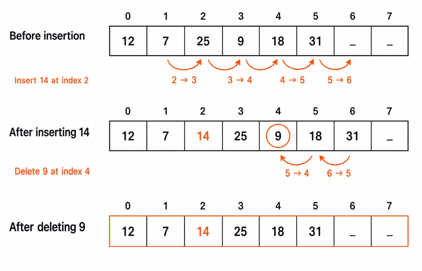
Start with capacity 8, logical size 6, and [12, 7, 25, 9, 18, 31, _, _]. To insert 14 at index 2, move elements from right to left so no value is overwritten:
The Queue Data Structure: Operations, Circular Queues and Worked Examples for GATE follows 12, 7, 25 and 9 through FIFO wraparound, while the Stack Data Structure: Operations, Applications and Worked Examples follows them through LIFO top changes. Array insertion and deletion ignore arrival order; indices decide which contiguous cells move.
Move
31from index5to6.Move
18from4to5.Move
9from3to4.Move
25from2to3.Write
14at index2.
The result is [12, 7, 14, 25, 9, 18, 31, _], logical size 7, after four shifts and one write.
Now delete index 4, value 9. Move 18 from 5 to 4, then 31 from 6 to 5. The result is [12, 7, 14, 25, 18, 31, _, _], logical size 6, with two shifts. Deleting a value also requires finding it unless its index is supplied.
Array access, traversal and search: when the complexity changes
Operation | Worst-case time | Reason or condition |
|---|---|---|
Indexed access |
| Direct address arithmetic |
Full traversal |
| Visit every element |
Linear search |
| Target may be last or absent |
Binary search |
| Input must be sorted |
Insert or delete at beginning or middle |
| Elements may need shifts |
Insert or delete at end |
| Capacity and target index already known |
Constant-time access comes from address arithmetic, not from arrays being small.
In [12, 7, 14, 25, 18, 31], linear search for 18 checks 12, 7, 14, 25, then 18, so it takes five comparisons. Binary search is invalid on this unsorted order.
After sorting to [7, 12, 14, 18, 25, 31], binary search for 18 checks index 2 (14), then index 4 (25), then index 3 (18). It succeeds in three comparisons. The sorted-input precondition is essential.
Fixed arrays, dynamic arrays and the linked-list trade-off
A language-level fixed array has a set capacity. A dynamic array abstraction can replace its backing storage when it becomes full. Suppose capacity 4 is filled by [3, 5, 8, 13]. Appending 21 requires capacity 8, copying all four existing values, and writing 21. Appending 34, 55 and 89 then uses spare cells without another resize.
The resize-triggering append is O(n), but append is amortised O(1) across many operations because copies are occasional.
Choice | Strength | Cost |
|---|---|---|
Array | Direct indexed access and cache-friendly contiguous storage | Middle updates shift elements; growth may reallocate |
Linked list | Relinking near a known node is convenient | Finding the kth element needs traversal and each node stores pointers |
Choose according to the access and update pattern.
Array mistakes that cost marks
Mistake | Consequence | Correction |
|---|---|---|
Confusing index with position | Off-by-one answer | State whether indexing begins at zero or another lower bound |
Dropping non-zero lower bounds | Wrong offset | Use |
Using rows in the row-major multiplier | Wrong address | Row-major counts complete rows of |
Applying binary search to unsorted data | Invalid reasoning | Sort first or use linear search |
Reading up to capacity | Accessing spare cells | Stop at logical size |
Calling every append worst-case | Ignores resizing | Distinguish one operation from amortised cost |
Use two quick checks. The first element must map to the base address, and adjacent elements in linear storage must differ by exactly w bytes. Substituting M[1][2] into either formula gives 2000. In the row-major sequence, M[1][3] is one four-byte cell later, at 2004.
Arrays in GATE and interview questions
IIT Guwahati's official GATE 2026 CS syllabus lists arrays in Section 4, Programming and Data Structures. The syllabus names topics only, so treat any weightage figure you see elsewhere as an estimate rather than an official number.
For exam practice, calculate both memory layouts before tracing an update, and state every complexity with its precondition.
For interviews, be ready to explain operation costs, trace an in-place update without losing data, identify an out-of-bounds bug, and choose an array or linked structure for a stated access pattern.
Array data structure: the short version and next step
Arrays use contiguous storage.
An address is the base plus an indexed offset.
Row-major counts complete rows; column-major counts complete columns.
Middle insertions and deletions shift elements.
Binary search requires sorted input.
Use GATE CS Exam Preparation Courses & Test Series for the broader subject path. GATE Guidance by Sanchit Sir is the structured next step if you want arrays sequenced with the rest of Programming and Data Structures. Otherwise, recompute both addresses and trace the shifts before moving on.
Keep learning
Tree Data Structure: Types, Traversals and a Worked BST Example
Build one nine-node binary search tree, classify its shape, trace four traversals, and work through insertion, search, deletion and complexity checks.
Updated 21 Oct 20266 min readDSA & Algorithms
Graphs in Data Structures: Complete Guide with BFS, DFS and Dijkstra Worked Examples
Learn graph terminology, representations and algorithm selection by tracing one unweighted graph with BFS and DFS, then solving a weighted graph with Dijkstra.
Updated 17 Oct 20266 min readDSA & Algorithms

Physical Security and Cryptography Basics: Controls, Keys and Worked Examples
Learn how physical and cryptographic controls work together, then apply them in a four-asset server-room model and a step-by-step toy RSA example.
Updated 13 Oct 20265 min readDSA & Algorithms
Stack Data Structure: Operations, Applications and Worked Examples
Build a stack from its LIFO rule, trace array and linked-list operations, evaluate a postfix expression, and practise recursion, applications, and common traps.
Updated 8 Oct 20265 min readDSA & Algorithms