Artificial Neural Networks Explained: Forward Pass, Worked Example and Exam Question Patterns
Build a small 2-2-1 neural network, calculate every value in its forward pass, and learn how activations, loss, training and parameter counts become exam tasks.
KnowledgeGate Team
Exam prep & CS education
Updated 25 Aug 20265 min read50 views
Neural-network terms sound intuitive until you must apply weights, biases and activations in the correct order. The 2-2-1 network below is traced from individual weighted sums through ReLU, sigmoid, classification loss and parameter counting. A feed-forward network is one type of artificial neural network; convolutional and recurrent networks use different connection patterns.
Related reading: perceptron backpropagation and activation function MCQs.
What an artificial neural network actually computes
An artificial neural network (ANN) is a directed network of simple computational units arranged in layers. The biological-neuron analogy explains the name, but the exam-ready definition is mathematical.
For one neuron with inputs , weights and bias :
\[
(z)
\]
Inputs are observed values. Weights control their influence, the bias shifts the decision boundary, and the activation function converts the linear total into the signal sent forward.
As a quick check, let , , and . Then . ReLU outputs . Without the bias, the output would be .
From one neuron to a feed-forward network
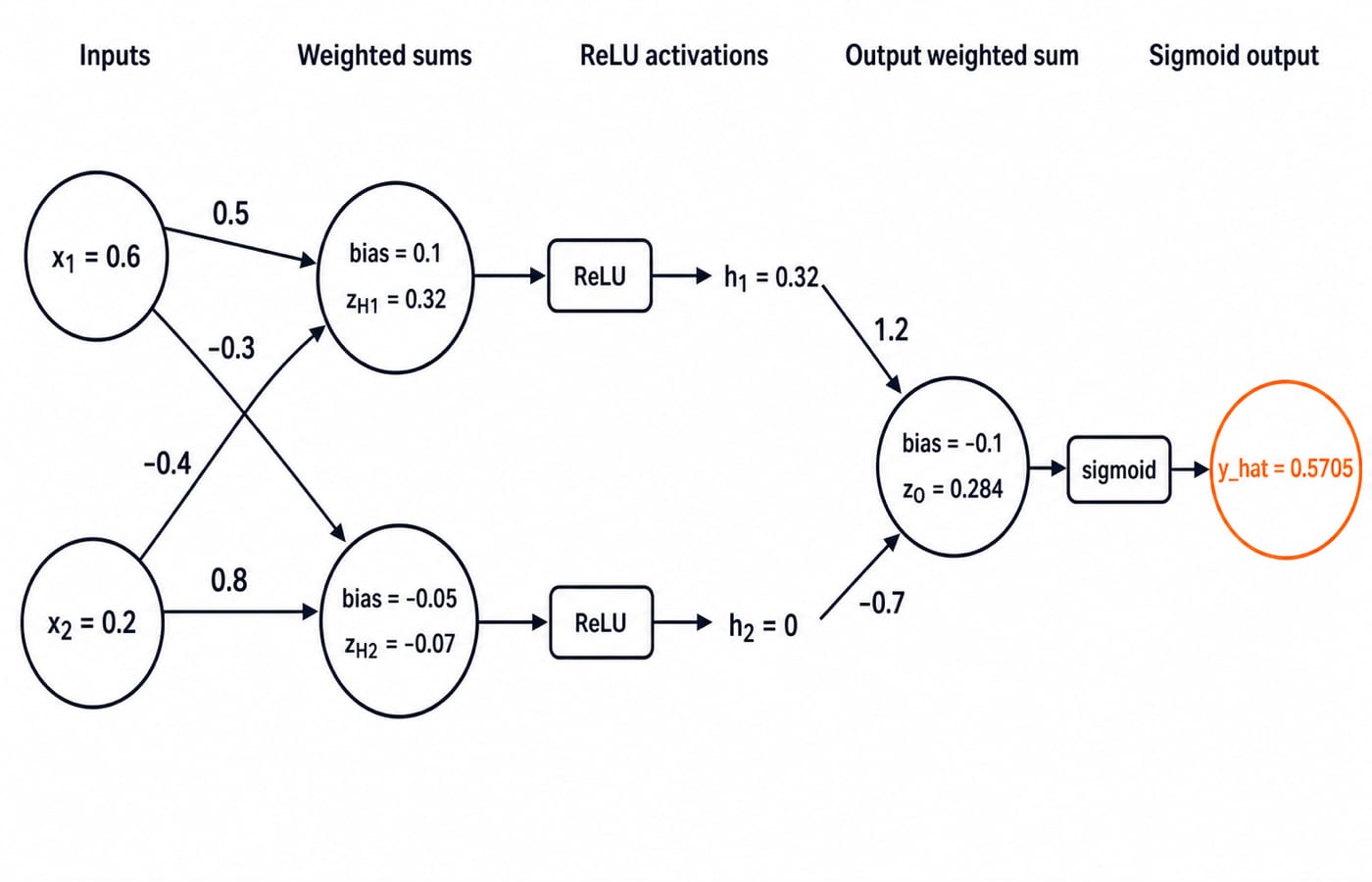
Our network has two input values, one hidden layer with two neurons, and one output neuron, written as a 2-2-1 architecture. The input layer stores values rather than calculating weighted sums. Feed-forward means the arrows do not loop back during this computation.
Layer count and connectivity define the architecture. Weights and biases are trainable parameters, while activations are intermediate results for one input. A single-layer perceptron has no hidden layer; a multilayer network has at least one. Backpropagation trains the parameters, but it does not change this forward calculation order. For a wider practical learning track, see the Skills category.
Worked example: calculate the complete forward pass
Calculate each hidden neuron before touching the output neuron:
\[
z_{H1}=(0.6)(0.5)+(0.2)(-0.4)+0.1=0.30-0.08+0.10=0.32
\]
Therefore, .
\[
z_{H2}=(0.6)(-0.3)+(0.2)(0.8)-0.05=-0.18+0.16-0.05=-0.07
\]
Therefore, .
Now pass and to the output neuron:
\[
z_O=(0.32)(1.2)+(0)(-0.7)-0.1=0.384-0.1=0.284
\]
\[
\hat y=\frac{1}{1+e^{-0.284}}=0.5705
\]
Unit | Weighted sum | Activation | Output |
|---|---|---|---|
H1 | 0.32 | ReLU | 0.32 |
H2 | -0.07 | ReLU | 0 |
O | 0.284 | Sigmoid | 0.5705 |
With a stated threshold of , the predicted class is . If the true label is , binary cross-entropy is . Loss measures how far the prediction is from the target under the chosen loss function.
The order is important. H2's negative pre-activation becomes zero before the output calculation, so its outgoing weighted term contributes nothing. Carrying forward instead would describe a different and incorrect network computation.
Activation functions and why the network needs them
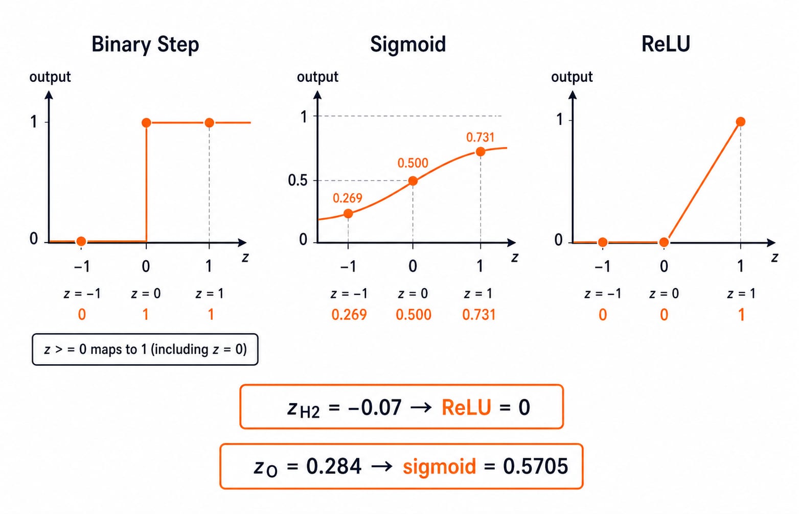
Use the convention stated in a question. Here, the binary step is for and for , sigmoid is , and ReLU is .
Function | Range | At | At | At | Introductory role |
|---|---|---|---|---|---|
Binary step | 0 | 1 | 1 | Hard decision | |
Sigmoid | 0.269 | 0.500 | 0.731 | Smooth binary output | |
ReLU | 0 | 0 | 1 | Hidden-unit activation |
ReLU suppresses H2 because . Sigmoid converts to , not directly to a class. Non-linearity matters because stacked linear transformations still collapse into one linear transformation. A multilayer network needs non-linear activations to model non-linear boundaries, though no activation is universally best.
How loss and gradients update the network
Training repeats five ordered moves:
Run a forward pass.
Compare the prediction with the target using a loss function.
Use backpropagation and the chain rule to obtain gradients.
Update parameters with gradient descent.
Repeat over training examples.
The update rule is . Here, is the current weight, the gradient describes how loss changes with that weight, and the learning rate controls the update size.
Conceptually, backpropagation follows the loss backwards through the output and hidden calculations. The chain rule combines each local rate of change, revealing how strongly each parameter affected the loss. A positive gradient makes gradient descent reduce the weight; a negative gradient makes it increase. With sigmoid output and binary cross-entropy, the output-logit gradient is ; hidden-layer gradients then multiply this signal by downstream weights and ReLU derivatives.
For our target and prediction , loss is about . If a later model produced a correct-class prediction of , loss would fall to . The value isolates the loss comparison; it is not the output of the stated weights.
A learning rate is the step size of an update. An epoch is one complete pass through the training set. Overfitting occurs when a model learns training examples too closely and performs poorly on unseen examples.
How exam questions turn ANN ideas into tasks
Common tasks ask you to identify components in a diagram, compute one neuron's output, trace a forward pass, match activations to ranges, count parameters, or notice whether a classification threshold is supplied.
Before calculating, mark the given activation beside each layer and write the threshold separately. This prevents two common category errors: applying the output activation inside the hidden layer, and treating a probability-like sigmoid output as a final class when no decision rule has been stated.
For the worked network, input-to-hidden weights contribute , hidden biases contribute , hidden-to-output weights contribute , and the output bias contributes . The total is trainable parameters. Input values and activations are not parameters.
The 2-2-1 trace isolates the exact layer-by-layer forward pass. Perceptron separability, a full gradient-descent update and multilayer parameter counting appear in Artificial Neural Networks: Worked Examples for GATE.
Common ANN calculation traps and their corrections
Trap | Correction |
|---|---|
Omit the bias | Add after all weighted input terms. |
Lose a negative weight's sign | Write each product in brackets before adding. |
Activate too early | Finish the full weighted sum , then apply . |
Pass through ReLU unchanged | ReLU of any negative input is . |
Turn sigmoid into a class immediately | Classify only after a threshold is supplied. |
Count input nodes or activations as parameters | Count only weights and biases. |
Treat weights as probabilities | Weights are learned influence coefficients and need not lie in . |
Call every neural network deep | Depth depends on the number of learned layers, not the presence of neurons. |
Keep four decimal places through sigmoid and loss calculations, then round at the end. At , copy the activation convention given in the question instead of assuming one.
The short version and the next calculation
Compute the weighted sum.
Add the bias.
Apply the activation.
Move layer by layer to the prediction.
Use loss to guide parameter updates.
The calculation chain is .
Now change only from to , keeping . The hidden sums become and , so and . Then , giving . At threshold , the class remains .
If you want a structured path from introductory AI concepts into machine learning and generative AI, continue with Artificial Intelligence (AI).
Keep learning
Problem Representation in AI: State Space, Worked Water-Jug Example and Exam Traps
Learn how states, operators, goals and costs turn a verbal task into a search problem. The worked water-jug trace separates valid states from reachable ones.
Updated 23 Oct 20265 min readML & Data Science
Foundations and Evolution of AI: Approaches, Timeline and a Worked Rational-Agent Example
Build a connected map of AI foundations, historical shifts and major paradigms, then calculate how a rational agent chooses under uncertainty.
Updated 19 Oct 20266 min readML & Data Science
Natural Language Processing Explained: Pipeline, TF-IDF Worked Example and Exam Patterns
Start from raw text, build BoW and TF-IDF vectors, compute cosine similarity, examine ambiguity, and finish with evaluation and exam-style checks.
Updated 15 Oct 20266 min readML & Data Science
Fundamentals of Planning in AI: STRIPS, State-Space Search and a Worked Blocks World Plan
Build a planning problem from facts, actions and goals, then follow every add and delete effect through a complete six-step Blocks World solution.
Updated 11 Oct 20266 min readML & Data Science