Relational Algebra for GATE: Operators, Tuple-Counting and Query Equivalence Drills
Calculate set, join, and outer-join cardinalities on concrete relations, then use selection and projection pushdown without changing query meaning.
KnowledgeGate Team
Exam prep & CS education
Updated 21 Jul 20266 min read
Relational algebra questions usually hide one of two jobs: count the result tuples, or decide whether two expressions always agree. Both jobs become easier when you stop reasoning from symbols alone and write a tiny relation instance. Four rows per relation is normally enough: once every matching pair is on paper, a counting question turns into arithmetic and an equivalence question turns into a hunt for one counterexample.
Core relational algebra operators
Relational algebra is closed: every operator takes relations as input and returns a relation. Its fundamental and commonly derived operators are:
Operator | Notation | Main effect |
|---|---|---|
Selection |
| Keeps rows satisfying a predicate |
Projection |
| Keeps columns and removes duplicate tuples |
Union |
| Keeps tuples in either compatible relation |
Difference |
| Keeps tuples in the left relation but not the right |
Cartesian product |
| Pairs every left tuple with every right tuple |
Rename |
| Renames a relation or its attributes |
Intersection |
| Keeps tuples present in both relations |
Join |
| Combines tuples that satisfy a match condition |
Division |
| Answers a "for every" condition |
Relational algebra uses set semantics. Projection removes duplicates. Plain SQL generally uses bag semantics, so SELECT dept may repeat values while relational pi_dept behaves like SELECT DISTINCT dept. The SQL queries and joins guide is the right companion when translating these operators into SQL.
Tuple-count bounds worth deriving
Let r contain m tuples and s contain n tuples. Assume union compatibility where required.
Expression | Minimum | Maximum |
|---|---|---|
|
|
|
|
|
|
|
|
|
|
|
|
|
|
|
For m=5 and n=3, union ranges from max(5,3)=5 to 5+3=8. Intersection ranges from 0 to 3. Difference r-s ranges from max(0,5-3)=2 to 5. Product is exactly 5x3=15.
Now verify those set operations on concrete unary relations P={1,2,3,4} and Q={3,4,5}:
P union Q = {1,2,3,4,5}, so the count is 5.P intersection Q = {3,4}, so the count is 2.P-Q = {1,2}, so the count is 2.Q-P = {5}, so reversing difference changes the count to 1.
Worked inner and outer joins
Use these relation instances:
R.A | R.B |
|---|---|
1 | x |
2 | y |
3 | y |
4 | z |
S.B | S.C |
|---|---|
x | 10 |
y | 20 |
y | 30 |
w | 40 |
The natural join matches on B. The R tuple (1,x) matches one S tuple. Each of (2,y) and (3,y) matches two S tuples. (4,z) matches none. Therefore the inner-join count is 1 + 2 + 2 + 0 = 5.
A | B | C |
|---|---|---|
1 | x | 10 |
2 | y | 20 |
2 | y | 30 |
3 | y | 20 |
3 | y | 30 |
For the left outer join, keep every R tuple and pad the unmatched one with NULLs. (4,z) has no partner in S, so it survives with a NULL C. Count: 5+1=6.
A | B | C |
|---|---|---|
1 | x | 10 |
2 | y | 20 |
2 | y | 30 |
3 | y | 20 |
3 | y | 30 |
4 | z | NULL |
The right outer join instead preserves the unmatched S tuple (w,40) and pads A with NULL, so its count is also 5+1=6. The full outer join preserves both unmatched tuples: 5+1+1=7.
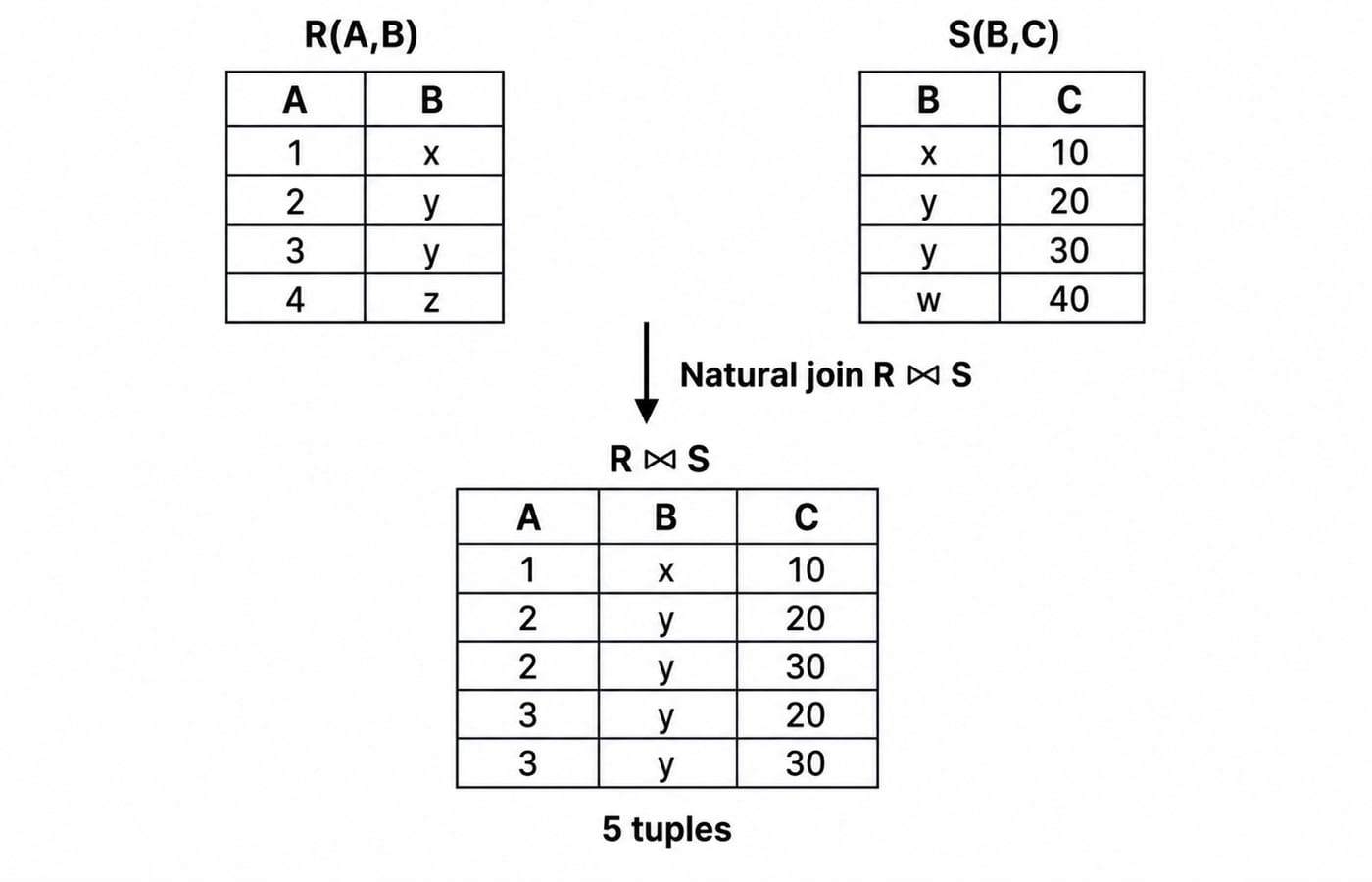
This example also shows why a join can exceed either input count. Repeated matching values create several combinations even though each input relation itself contains no duplicate tuple.
Join counts under key constraints
Suppose S.B is a primary key and every R.B is a non-NULL foreign key referencing it. Each R tuple matches exactly one S tuple, so R natural join S has exactly m tuples. If the foreign key is nullable or unenforced, some R tuples may not match, and the count can fall below m.
If two relations share no attribute, a natural join has no equality condition and becomes their Cartesian product, with exactly mn tuples. If a question gives only m and n without key, foreign-key, or value-frequency information, do not invent an exact inner-join count. Use the valid range 0 to mn.
Division means "for all"
If Enrolled(student, course) records enrolments and Required(course) lists required courses, then Enrolled division Required returns students enrolled in every required course. One standard construction is:
pi_student(Enrolled) - pi_student((pi_student(Enrolled) x Required) - Enrolled)
The inner difference finds missing student-course pairs. Projecting gives students who miss something. Subtracting them leaves only students with all required pairs.
Query equivalence and safe pushdown
Selection cascades and commutes:
sigma_p(sigma_q(R)) = sigma_q(sigma_p(R)) = sigma_(p AND q)(R).
Selection also pushes through a join when its predicate refers only to one input:
sigma_p(R join S) = sigma_p(R) join S, when p uses only R attributes.
Projection pushdown needs more care. You may remove unused attributes early, but each side must retain its join attributes plus every attribute needed later. Projecting away the join column before the join makes the rewrite wrong or undefined. Selection and projection commute only when the projected attributes retain every attribute mentioned by the selection predicate.
A theta join is a selected Cartesian product:
R join_condition S = sigma_condition(R x S).
For a natural join, equal-name attributes form the equality conditions, followed by a projection that keeps one copy of each common attribute. Rename first when a self-join or same-name collision would make the condition ambiguous.
One classic non-equivalence is projection over difference. Let R={(1,a),(2,b)} and S={(1,b)}. Then R-S=R, so projecting A gives {1,2}. But pi_A(R)-pi_A(S)={1,2}-{1}={2}. Two tuples on the left and one on the right are enough to show that projection does not distribute over difference.
Relational algebra drills: tuple counts and rewrites
Work these on paper before reading the answers. Drills 2 and 4 reuse the relations R and S given earlier.
rholds 8 tuples andsholds 5, and the two are union compatible. Give the full range forr union sand forr-s.Add the tuple
(5,y)to R, leave S unchanged, and recount all four joins: natural, left outer, right outer, full outer.R holds 12 tuples, S holds 7,
S.Bis a primary key, and everyR.Bis a non-NULL foreign key into it. How many tuples doesR natural join Sreturn? Then answer the same question for two relations that share no attribute name at all.Is
sigma_(C>15)(R join S) = R join sigma_(C>15)(S)? Decide from the pushdown rule first, then check it by listing both result sets.
Answers
r union sruns frommax(8,5)=8, when every s tuple already sits in r, up to8+5=13when the two are disjoint.r-sruns frommax(0,8-5)=3up to 8.(5,y)matches(y,20)and(y,30), so the natural join gains two rows:5+2=7.(4,z)is still the only unmatched R tuple, so the left outer join is7+1=8.(w,40)is still the only unmatched S tuple, so the right outer join is also7+1=8. The full outer join is7+1+1=9.Exactly 12. Each R tuple matches exactly one S tuple, so the join neither drops nor duplicates a row, and the answer does not depend on S holding 7 tuples. With no shared attribute the natural join degenerates to a Cartesian product:
12x7=84.Yes. The predicate names only C, an S attribute, so it may be pushed onto S. Filtering the five join rows leaves
(2,y,20),(2,y,30),(3,y,20)and(3,y,30), and joining R withsigma_(C>15)(S) = {(y,20),(y,30)}produces the same four rows.
How GATE tests relational algebra
Expect exact or extreme tuple counts, translation between algebra and SQL, and equivalent-expression choices. On a counting question, list matches by join value. On an equivalence question, apply a valid law or build the smallest counterexample that breaks it, usually two or three tuples. The DBMS normalization explained post is the natural next DBMS topic once algebra is solid.
About 2,100 Database Management System questions sit in the KnowledgeGate question bank when you want broader practice across the rest of the subject. Confirm current paper instructions on the official GATE portal of the organising IIT.
The short version
Derive set-operation bounds from overlap, count joins from actual matching groups, and add unmatched rows only for the preserved side of an outer join. For equivalence, push selection freely only when its attributes belong to that input, and push projection only while retaining join and output attributes.
Redo the four drills cold, without looking at the answers. Then use the GATE Test Series under time pressure, and the GATE category page to choose the next practice block.
Keep learning

SQL Joins Explained: INNER, LEFT, RIGHT, FULL, CROSS and SELF with Runnable Examples
Trace all six SQL join types on one support-agent dataset, with runnable queries, exact outputs, NULL behaviour, row counts and filter-placement traps.
Updated 21 Oct 20265 min readDBMS
GROUP BY and HAVING in SQL: Syntax and Worked Examples
Trace eight sales rows through WHERE, GROUP BY, aggregates, and HAVING, then tackle multiple columns, NULLs, COUNT variants, and common query traps.
Updated 17 Oct 20265 min readDBMS

SQL Aggregate Functions: COUNT, SUM, AVG, MIN and MAX with Examples
Use one runnable sales table to see exactly how SQL aggregates treat rows, NULL values, duplicates and groups. Every result includes the arithmetic behind it.
Updated 13 Oct 20265 min readDBMS

Query Languages in DBMS: Relational Algebra, SQL and a Worked Query
Follow one database request from plain English to relational algebra, intermediate relations, relational calculus and SQL, with every result traced.
Updated 9 Oct 20265 min readDBMS