A process is more than a program file, and process management is more than choosing the next CPU burst. The operating system creates processes, records state, queues them, dispatches the CPU, handles waits, and collects terminated processes. One control loop links states and the PCB to FCFS and Round Robin calculations.
Process management in an operating system: the complete control loop
A program is executable code on disk. A process is an execution instance with an identifier, current instruction, registers, address space, stack, resources, and scheduling state. Two processes can run the same program with separate contexts.
The kernel creates and schedules processes, tracks states, switches contexts, blocks and wakes processes, coordinates interactions, and cleans up after termination. GATE CS Exam Preparation provides the wider subject route.
In a Unix-style lifecycle, parent PID 4200 creates child PID 4201. The child loads sort, exits with status 0, and the parent calls wait to collect that status and release the process-table entry. A terminated child awaiting collection is a zombie, not an orphan.
Process states and transitions: follow one process through the system
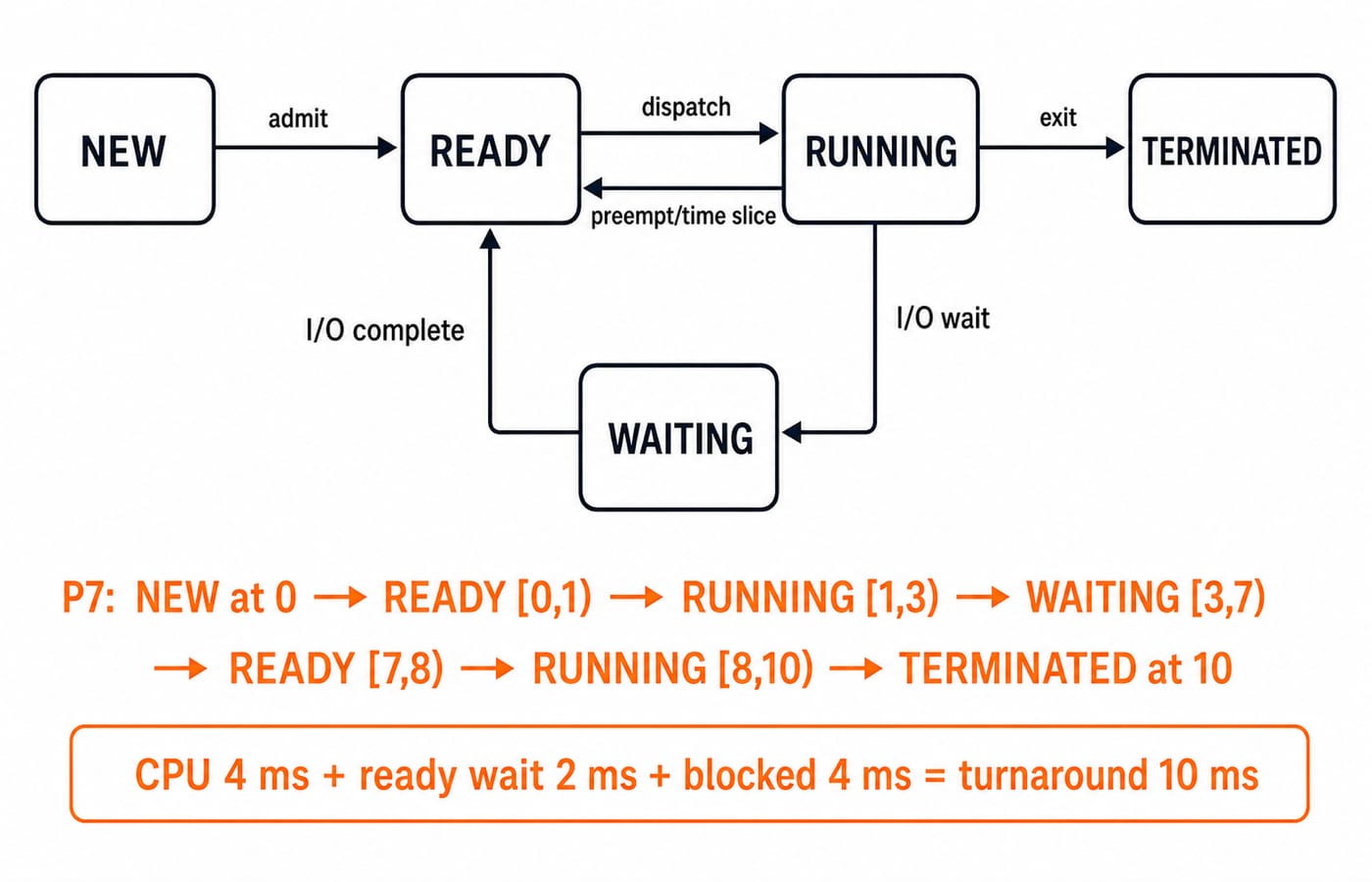
The five-state model has these transitions:
NEW -> READY: admit.READY -> RUNNING: dispatch.RUNNING -> READY: preemption or time-slice expiry.RUNNING -> WAITING: I/O or event wait.WAITING -> READY: I/O or event completion.RUNNING -> TERMINATED: exit.
READY means able to run but awaiting the CPU. WAITING, also called BLOCKED, means unable to proceed until an event.
Process P7 arrives at t=0 ms and needs two 2 ms CPU bursts separated by 4 ms of disk I/O. It enters READY at t=0, dispatches at t=1, and runs on [1,3). Its disk request puts it in WAITING on [3,7). Completion returns it to READY at t=7; dispatch at t=8 runs it on [8,10) before exit at t=10.
CPU time is 2 + 2 = 4 ms; ready wait is 1 + 1 = 2 ms; blocked time is 4 ms; turnaround is 10 - 0 = 10 ms. Check: 4 + 2 + 4 = 10 ms.
The seven-state model adds READY SUSPENDED and BLOCKED SUSPENDED when a medium-term scheduler removes processes from memory. Suspension is not blocking. For classification practice, use Process Management & Process States MCQs.
Process control block and context switch: what the OS saves
The PCB lets the kernel resume a process.
Field group | Example value for P7 | Purpose |
|---|---|---|
Identity |
| Identifies the process |
State |
| Tracks lifecycle position |
Saved CPU context | PC | Enables resumption |
Scheduling data | Priority, queue pointers, CPU time | Supports selection |
Memory data | Page-table pointer | Locates address space |
I/O and accounting | Open resources, usage data | Tracks resource use |
P7's I/O request traps at t=3 ms. The kernel saves its context, marks it WAITING, and restores another ready process. The disk interrupt makes P7 READY at t=7; dispatch restores it at t=8.
A context switch is not merely a state change. It costs time without completing user work. Its duration varies, and a kernel entry need not switch processes.
Process schedulers, queues and the dispatcher
Processes use job, ready, and device or event queues. The long-term scheduler admits jobs and controls multiprogramming. The short-term scheduler selects from the ready queue. A medium-term scheduler suspends and resumes processes. The dispatcher performs the hand-off through context switching, required mode changes, and control transfer.
In P7's trace, admission at t=0 is a long-term decision in this teaching model. Choosing P7 at t=1 and t=8 is short-term scheduling. Moving it to the disk queue at t=3 and back to ready at t=7 is event-driven state management, not another admission.
This is a policy-mechanism split. The scheduling algorithm chooses a READY process; the dispatcher performs the switch. A scheduler cannot select a process still blocked on I/O.
CPU scheduling algorithms and the metrics they optimise
Algorithm | Selection rule | Preemptive? | Characteristic trade-off |
|---|---|---|---|
FCFS | Earliest arrival first | No | Simple, but long jobs delay shorter ones |
SJF | Shortest next burst | No | Low average wait, but long jobs can starve |
SRTF | Least remaining burst | Yes | Responds to short arrivals, with more preemption |
Priority | Highest priority first | Either | Expresses importance, but can starve low priorities |
Round Robin | Ready-queue order for one quantum | Yes | Improves sharing and response, with quantum-sensitive overhead |
SJF's minimum-average-waiting result assumes known or estimated burst lengths. RR depends on its time quantum. SJF-family and priority policies need ageing or another mechanism to prevent starvation.
For one CPU burst, define arrival time AT, burst time BT, completion time CT, turnaround time TAT = CT - AT, waiting time WT = TAT - BT, and response time RT = first CPU start - AT. Response time is not completion time, and waiting excludes CPU service.
No scheduler is universally best. Better response or fairness can increase average waiting or switching overhead, as this calculation shows.
FCFS and Round Robin worked example with exact Gantt charts
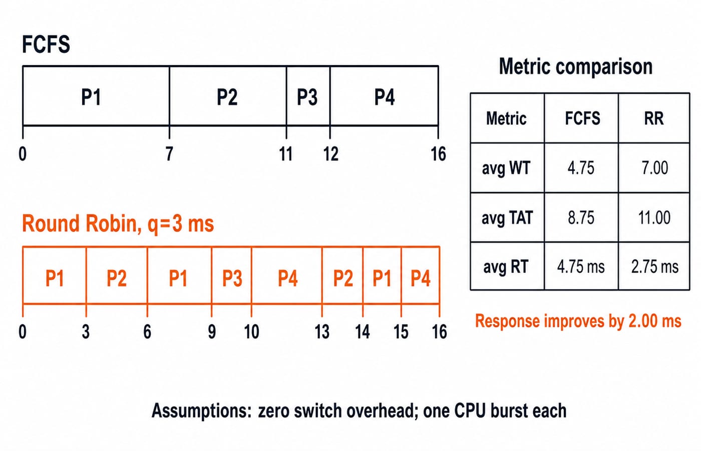
Assume one CPU burst each for P1(AT=0, BT=7), P2(AT=2, BT=4), P3(AT=4, BT=1), and P4(AT=5, BT=4). Time is in milliseconds, context-switch overhead is zero, there is no I/O, and Round Robin uses q=3 ms. Arrivals join the ready queue as they occur.
FCFS follows arrival order:
0-7 P1 | 7-11 P2 | 11-12 P3 | 12-16 P4
Process | CT | TAT = CT - AT | WT = TAT - BT | RT |
|---|---|---|---|---|
P1 | 7 | 7 | 0 | 0 |
P2 | 11 | 9 | 5 | 5 |
P3 | 12 | 8 | 7 | 7 |
P4 | 16 | 11 | 7 | 7 |
Average WT = (0+5+7+7)/4 = 19/4 = 4.75 ms, average TAT = (7+9+8+11)/4 = 35/4 = 8.75 ms, and average RT = (0+5+7+7)/4 = 19/4 = 4.75 ms.
For RR, each unfinished process returns to the queue after using at most 3 ms:
0-3 P1 | 3-6 P2 | 6-9 P1 | 9-10 P3 | 10-13 P4 | 13-14 P2 | 14-15 P1 | 15-16 P4
Process | CT | TAT | WT | First start | RT |
|---|---|---|---|---|---|
P1 | 15 | 15 | 8 | 0 | 0 |
P2 | 14 | 12 | 8 | 3 | 1 |
P3 | 10 | 6 | 5 | 9 | 5 |
P4 | 16 | 11 | 7 | 10 | 5 |
Average WT = (8+8+5+7)/4 = 28/4 = 7.00 ms; average TAT = (15+12+6+11)/4 = 44/4 = 11.00 ms; average RT = (0+1+5+5)/4 = 11/4 = 2.75 ms.
On this workload, FCFS has lower average waiting and turnaround, while RR improves average response from 4.75 to 2.75 ms, a 2.00 ms reduction. Under the stated counting convention, RR has seven process-to-process changes across eight slices; FCFS has three. This is a workload-specific trade-off, not proof that FCFS is generally superior.
Process management traps and how exams and interviews test them
Keep the distinctions precise: a program is not a process; READY is not WAITING; I/O completion normally moves a process to READY, not directly to RUNNING; the scheduler selects, while the dispatcher performs. A context switch is overhead, not useful CPU time. Turnaround, waiting, and response differ. A zombie has terminated but has not been reaped.
Common questions ask for the state after an event, a legal transition, a PCB field's purpose, or the scheduler that acts. Numericals require a Gantt chart and CT, TAT, WT, and RT. Others test starvation, ageing, process creation, threads, and context switching.
Use a 60-second routine: state assumptions, enqueue by arrival, draw every boundary, derive CT, then calculate TAT, WT, and RT. Verify elapsed CPU time. Both charts end at 16 ms, equal to 7+4+1+4, because overhead and idle time are zero.
After lifecycle and scheduling, study Process Synchronization and Semaphores for concurrent processes sharing data. Synchronisation and scheduling differ.
Process management: the short version and next step
Use this mental model:
The PCB records.
States describe readiness.
Queues organise waiting.
The scheduler chooses.
The dispatcher switches.
P7 accounts for 4 + 2 + 4 = 10 ms, and both charts account for 16 ms of CPU work. For concept-led CS study, use GATE Guidance by Sanchit Sir. For timed practice, use the GATE Test Series. Then redraw both diagrams from memory, recompute every metric, and explain in one sentence why RR improves response here while increasing average waiting.