Image Fundamentals Explained: Sampling, Quantisation and Worked Examples
Follow one grayscale image from its pixel grid and histogram to downsampling, 2-bit quantisation, reconstruction error, neighbourhoods and distance measures.
KnowledgeGate Team
Exam prep & CS education
Updated 30 Aug 20266 min read
Students often call every array of numbers an image without separating the scene, the sampled pixel grid and the quantised code stored at each location. That leads to errors such as treating image dimensions as bit depth, treating fewer grey levels as fewer pixels, or believing a histogram preserves spatial arrangement. Keeping the same 4 x 4 values makes the distinctions concrete: the grid has 16 spatial samples, each stored as one 8-bit code before any downsampling or quantisation.
Build the right mental model: scene, samples and stored codes
A continuous image such as f(x,y) has continuous coordinates and amplitude. Spatial sampling selects finite locations, while amplitude quantisation maps measurements to finite codes:
scene -> sensor measurement -> spatial samples -> quantised codes -> stored array
Binary images commonly use two codes. An 8-bit grayscale image has 2^8 = 256 levels, 0 through 255. Three 8-bit RGB channels need 3 x 8 = 24 raw bits per pixel. A pixel is a sampled location plus its value or tuple, not a physical square of universal size.
An array alone does not specify pixel spacing, colour interpretation, transfer characteristics or compression. These need conventions or metadata. Image arrays are matrices, so their transformations reuse the notation and operations of Linear Algebra for GATE CS.
Separate spatial resolution, grey-level resolution and storage
Use x = column left to right and y = row top to bottom, with (0,0) at top left. For M rows and N columns, 0 <= x < N and 0 <= y < M. Other origins and axis directions exist, so declare the convention.
Spatial resolution is the sample grid, such as 4 x 4; bit depth controls codes per channel. With k bits, L = 2^k, while at least L codes need ceil(log2 L) bits. You can revise powers of two and binary code counts separately.
Raw sample storage is:
rows x columns x channels x bits per channel
Our image needs 4 x 4 x 1 x 8 = 128 bits = 16 bytes. A 1024 x 768 8-bit grayscale array needs 786,432 bytes = 0.75 MiB; 24-bit RGB needs 2,359,296 bytes = 2.25 MiB. With 1 MiB = 1,048,576 bytes, these raw amounts exclude headers, row padding, metadata and compression.
Worked example, part 1: coordinates, values and histogram
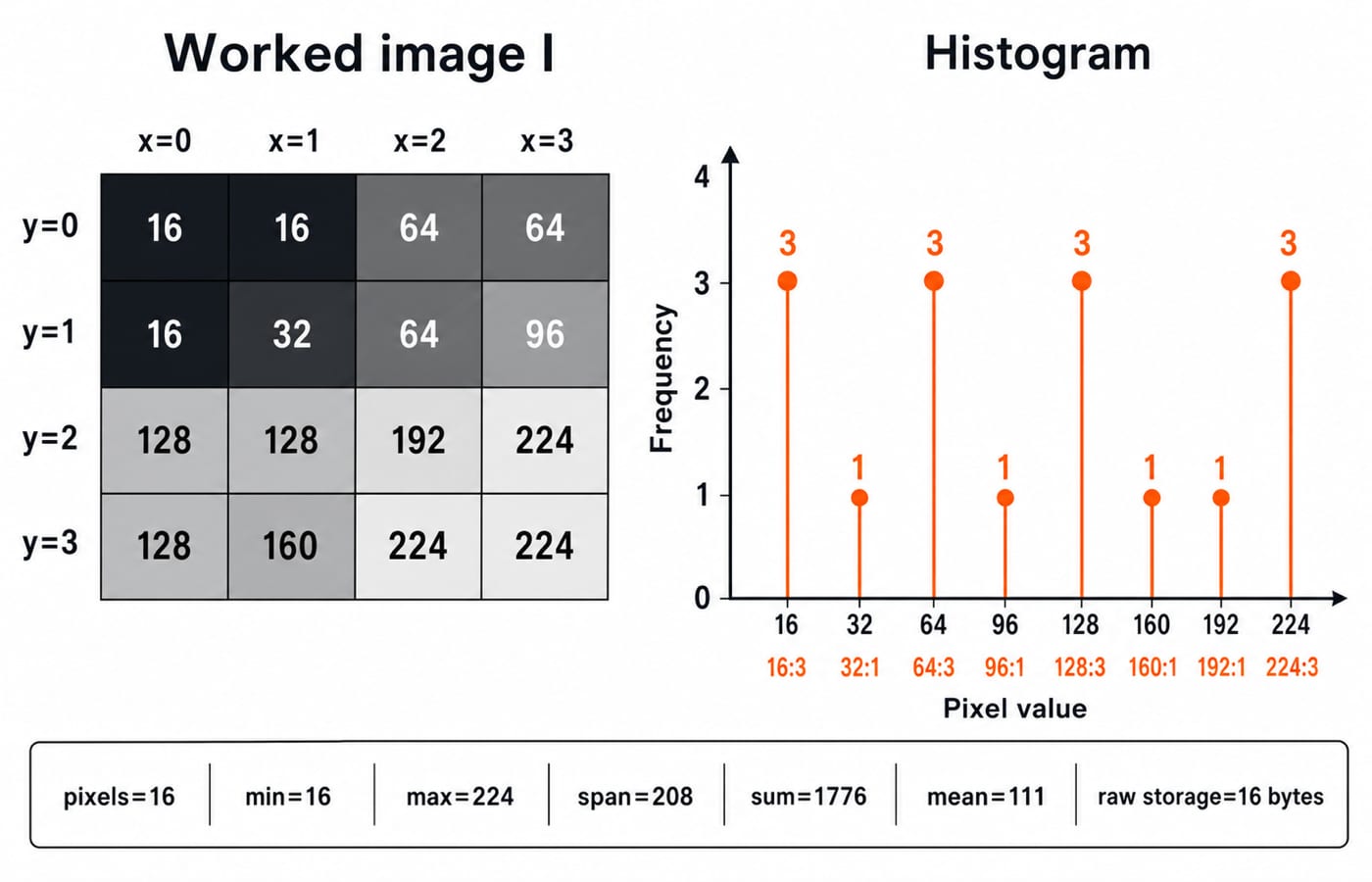
Write rows from y=0 to y=3, and entries in each row from x=0 to x=3:
I = [ [ 16,  16,  64,  64],
      [ 16,  32,  64,  96],
      [128, 128, 192, 224],
      [128, 160, 224, 224] ]
Here I(0,0)=16, I(1,1)=32, I(2,1)=64, I(1,2)=128 and I(3,3)=224. There are 16 pixels, minimum 16, maximum 224, span 224 - 16 = 208, and eight observed values, although 256 codes remain possible.
Intensity | 16 | 32 | 64 | 96 | 128 | 160 | 192 | 224 |
|---|---|---|---|---|---|---|---|---|
Histogram | 3 | 1 | 3 | 1 | 3 | 1 | 1 | 3 |
Other codes have count zero. Check 3+1+3+1+3+1+1+3 = 16. The sum is 3(16)+32+3(64)+96+3(128)+160+192+3(224) = 1776, giving mean 1776/16 = 111.
A histogram keeps frequencies, not locations. Rearranging the 16 entries preserves these counts and the mean but changes the spatial image.
Worked example, part 2: change sampling, not quantisation
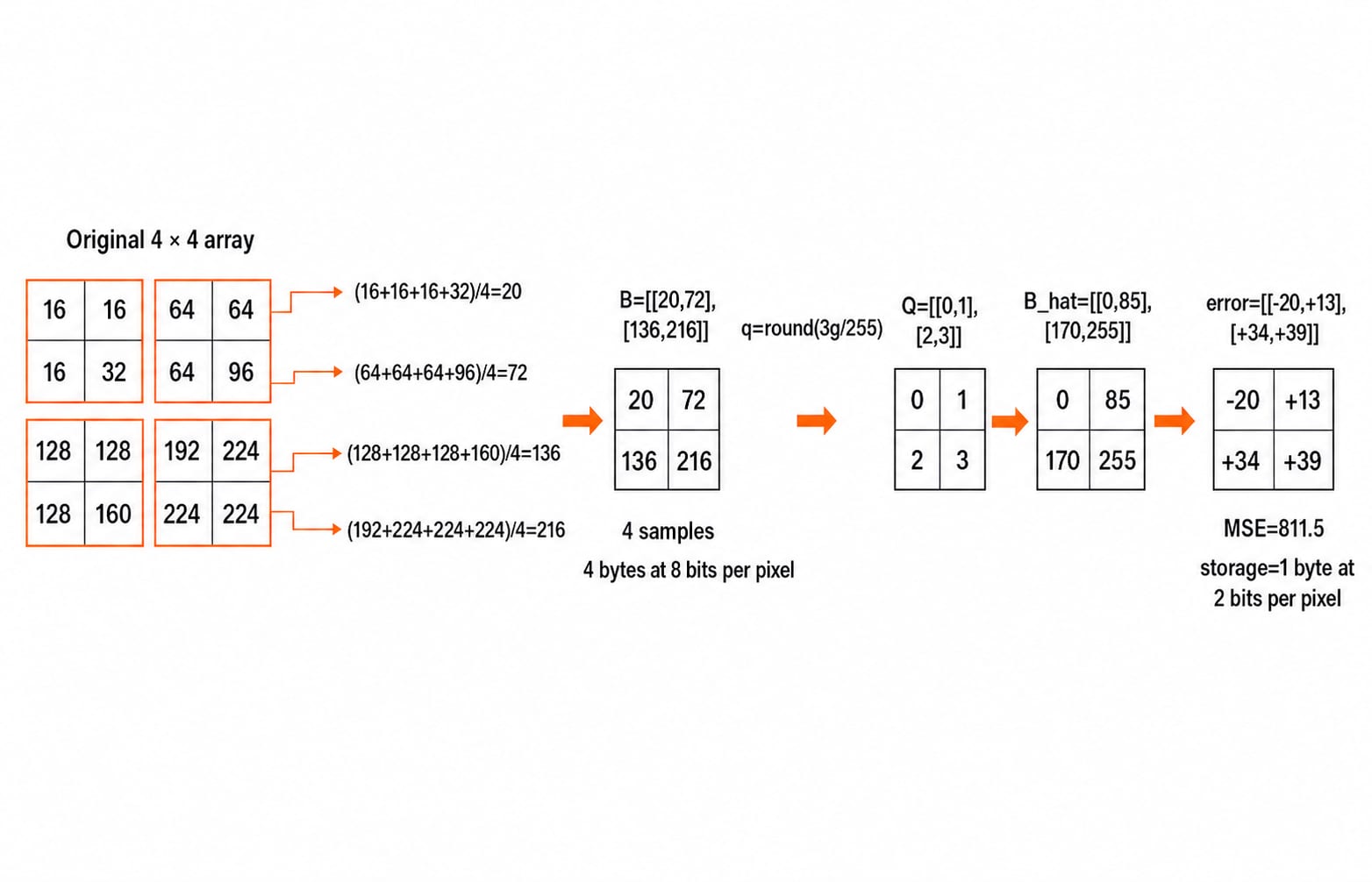
Downsample I to 2 x 2: split it into non-overlapping 2 x 2 blocks, replace each block by its mean, and keep the field of view fixed.
B(0,0) = (16+16+16+32)/4 = 80/4 = 20B(1,0) = (64+64+64+96)/4 = 288/4 = 72B(0,1) = (128+128+128+160)/4 = 544/4 = 136B(1,1) = (192+224+224+224)/4 = 864/4 = 216
Thus B=[[20,72],[136,216]]. Samples fell from 16 to 4, one quarter, while the means still fit 8-bit codes. At fixed field of view, spacing doubles on both axes. Block averaging plus decimation is illustrative, not universal.
A 4 x 4 checkerboard alternating 0 and 255 becomes all-zero 2 x 2 if only even-row, even-column samples remain. Averaging each 2 x 2 block gives 127.5, rounded to 128. This shows why phase and prefiltering matter, although block averaging cannot remove all aliasing.
Worked example, part 3: quantise and measure error
Keep the 2 x 2 grid fixed but reduce amplitude precision to 2 bits. Use q = round(3g/255), for q in {0,1,2,3}, and reconstruct with g_hat = 85q.
20 -> q=0 -> 072 -> q=1 -> 85136 -> q=2 -> 170216 -> q=3 -> 255
So Q=[[0,1],[2,3]] and B_hat=[[0,85],[170,255]]. Define signed error as reconstructed minus original. The error matrix is [[-20,+13],[+34,+39]].
MSE = [(-20)^2 + 13^2 + 34^2 + 39^2]/4
= (400 + 169 + 1156 + 1521)/4
= 3246/4 = 811.5
MSE depends on reconstruction and is not a wrong-pixel count. At 8 bits, B needs 4 x 8 = 32 bits = 4 bytes; at 2 bits, 4 x 2 = 8 bits = 1 byte. The original 16-to-1 byte drop reflects fewer samples and lower amplitude precision, not quantisation alone.
Use neighbourhoods, adjacency and distance consistently
For p=(1,1)=32, the 4-neighbours are (1,0)=16, (0,1)=16, (2,1)=64 and (1,2)=128. The diagonals are (0,0)=16, (2,0)=64, (0,2)=128 and (2,2)=192; their union is the 8-neighbourhood. Border pixels have fewer valid neighbours because coordinates outside 0..3 are absent.
For r=(2,2)=192, p and r are 8-adjacent but not 4-adjacent when values are ignored. Under V={32,192}, they are m-adjacent because common 4-neighbours (2,1)=64 and (1,2)=128 contain no value from V. Value-restricted adjacency uses the set supplied.
For p=(1,1) and s=(3,2), D4=|3-1|+|2-1|=3, D8=max(2,1)=2, and DE=sqrt(2^2+1^2)=sqrt(5), about 2.236. These are coordinate distances; intensity difference is |224-32|=192.
Image-fundamentals traps and practice checks
Trap | What goes wrong | Correct check | Worked evidence |
|---|---|---|---|
Swap row and column | Wrong pixel | Apply |
|
Change origin | Locations shift | Declare | Top left is 16 |
Call | Grid and codes mix | Separate dimensions, bits | 16 pixels, 8 bits each |
Assume 256 codes occur | Capacity becomes observation | Count values | Eight occur |
Write | Codes become bits | Use | 256 codes, 8 bits |
Forget bits-to-bytes | Eightfold overcount | Divide by 8 | 128 bits is 16 bytes |
Treat file size as raw storage | Overheads vanish | Label raw storage | Headers excluded |
Equate fewer samples with fewer levels | Reductions mix | Track grid and depth |
|
Omit quantiser rules | Result is irreproducible | State both rules |
|
Round means early | Arithmetic drifts | Finish each mean | Last block is 216 |
Assign histogram locations | Order is invented | Keep counts only |
|
Ignore allowed values | Adjacency changes | Apply stated | m-adjacent for |
Exam-style practice may ask for I(2,1)=64, 16 raw bytes, h(224)=3, mean 111, B, Q, MSE 811.5, four neighbours, or three distances. Recompute each result without notes and isolate any slow definition before moving on.
Image fundamentals: the short version and next step
Start by declaring the coordinate convention and separating the continuous scene from its sampled grid. Record rows, columns, channels and bits per channel, then compute raw storage in bits before converting to bytes. Keep sampling separate from quantisation, and state every averaging, rounding and reconstruction rule. Finally, choose the required neighbourhood or distance definition.
Without notes, recover for I: 16 pixels, 16 raw bytes, minimum 16, maximum 224, mean 111 and h(64)=3. Then recover B=[[20,72],[136,216]], Q=[[0,1],[2,3]], B_hat=[[0,85],[170,255]], error [[-20,+13],[+34,+39]] and MSE 811.5. For a structured route that includes Computer Graphics, use ZERO TO HERO (Complete Course), or browse the wider CS Fundamentals catalogue.
Keep learning
NOT, OR and AND Gates: Evolution, Truth Tables and a Worked Circuit
Learn how NOT, OR and AND gates developed from switching ideas, then trace F=(A+B')C node by node and confirm it with a complete truth table.
Updated 23 Oct 20265 min readDigital Logic
Binary Arithmetic Operations Explained: Rules and Worked Examples
Learn binary addition, subtraction, multiplication and division with aligned worked examples, then separate carry, borrow and two's-complement overflow.
Updated 19 Oct 20266 min readDigital Logic
1's Complement Explained: Binary Conversion, Addition and Worked Examples
Learn how fixed-width 1's complement numbers represent negatives, why zero has two encodings, and how end-around carry works through exact examples.
Updated 15 Oct 20266 min readDigital Logic
Decimal Conversion Explained: Binary, Octal and Hexadecimal Worked Examples
Learn one dependable method for converting values between decimal, binary, octal and hexadecimal, including fractions, shortcuts and checks.
Updated 11 Oct 20265 min readDigital Logic