One-to-One (Injective) Function: Definition, Counting Formula, Properties and Worked Examples

Many students confuse two different requirements: a function gives one output for every input, while an injective function gives different outputs to different inputs. That distinction controls both identification questions and counting problems. The collision test works for mappings, formulas and tables, and the count is n!/(n-m)!, including the zero-count case. Injectivity connects with bijections, and composition and inverse-on-image properties follow from it. You can place this topic inside the wider GATE CS exam preparation path.

1. One-to-one function definition and the collision test

Let f:A->B be a function. It is one-to-one, or injective, if for every x1,x2 in A,

f(x1)=f(x2) implies x1=x2.

Equivalently, if x1!=x2, then f(x1)!=f(x2). This is the collision test: two distinct domain elements must never share an image. Injectivity does not require every element of the codomain to be used. For the total-function rule and unrestricted count n^m, use Definition of a Function: Domain, Codomain, Range and Counting Formula. Injective counting begins when the no-collision constraint replaces independent choices.

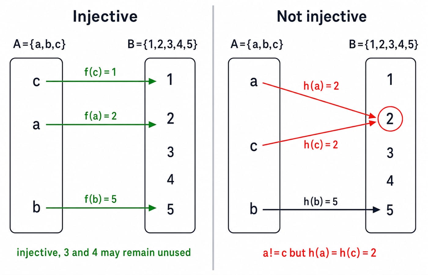
Take A={a,b,c} and B={1,2,3,4,5}. Define f(a)=2, f(b)=5 and f(c)=1. The images 2,5,1 are all different, so f is injective. The unused values 3 and 4 do not create a problem.

Now define h(a)=2, h(b)=5 and h(c)=2. Here a!=c, but h(a)=h(c)=2. That single collision proves that h is not injective.

2. Number of one-to-one functions between finite sets

Suppose |A|=m and |B|=n. Assign images to the elements of A one at a time. The first input has n choices. Once that image is used, the second input has n-1 choices. Continuing without replacement, the mth input has n-m+1 choices.

Therefore, when m<=n, the number of injective functions is

nPm=n(n-1)...(n-m+1)=n!/(n-m)!.

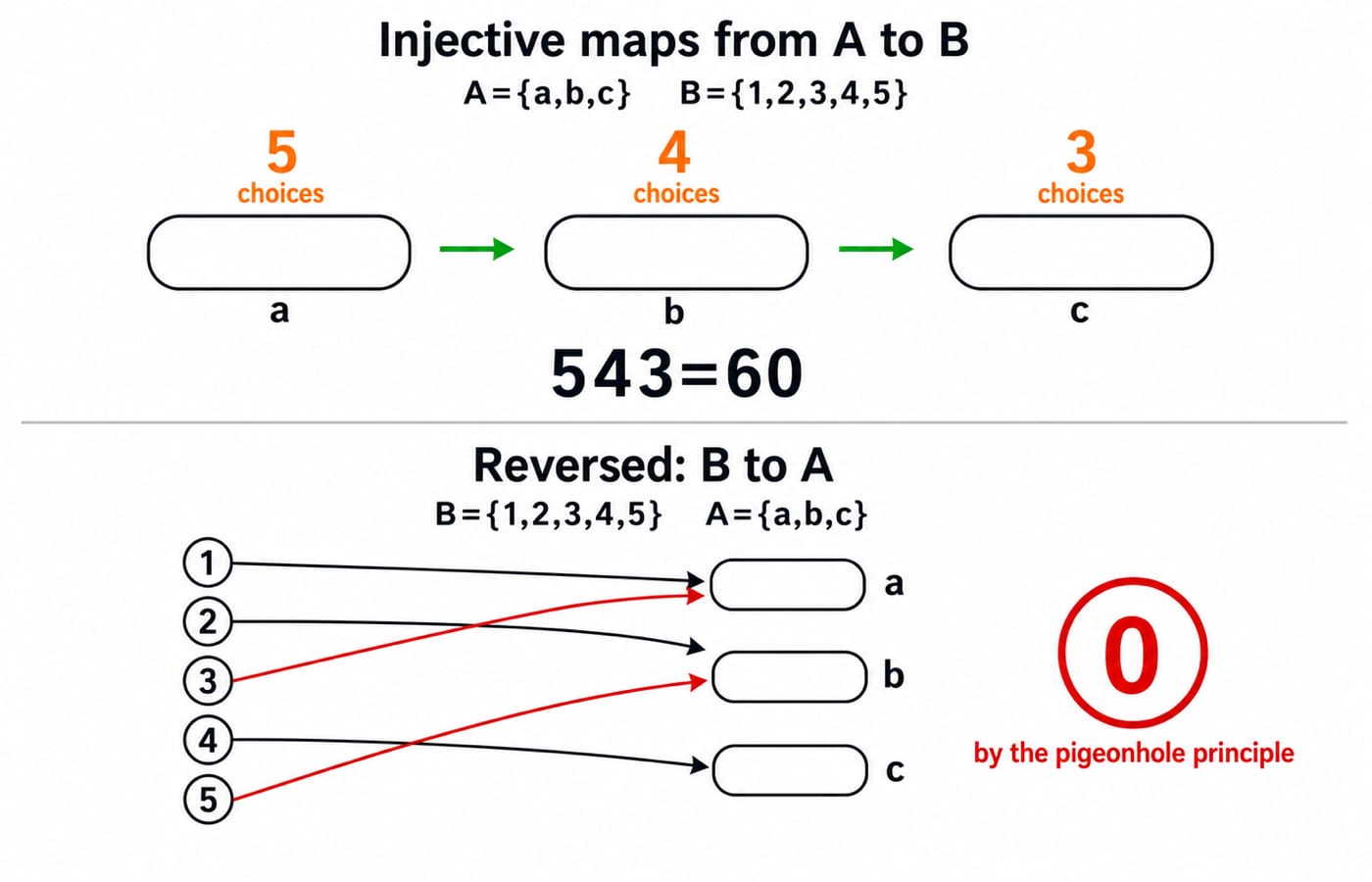
If m>n, the count is 0. By the pigeonhole principle, more inputs than outputs force at least two inputs to share an output. There is also a useful boundary case: if m=0, the empty domain has exactly one function to any codomain, and the formula gives n!/n!=1.

For A={a,b,c} and B={1,2,3,4,5}, choose f(a) in 5 ways, f(b) from the 4 unused values, and f(c) from the remaining 3. Thus

5P3=5*4*3=60.

In the reversed direction, an injective function from the five-element set B to the three-element set A is impossible. Its count is 0, not 3P5.

3. Counting injective functions with restrictions

Now keep the same sets and impose f(a)!=1. The image of a has 4 allowed choices. After choosing it, exactly one of the five codomain values has been used, so f(b) still has 4 choices. Then f(c) has 3 choices. The count is

4*4*3=48.

Notice why the two factors of 4 mean different things. The first excludes the forbidden value 1; the second excludes the value already assigned to a. No output is reused.

For another restriction, count injective functions whose image contains 5. Begin with all 60 injective functions. Those avoiding 5 must choose three distinct images from {1,2,3,4}, so their number is

4P3=4*3*2=24.

Hence the required count is

60-24=36.

Direct multiplication is usually clean when a condition fixes or forbids an early image. Complementary counting is often cleaner when the image must contain a specified codomain value.

4. Injective, surjective and bijective functions are different claims

These properties answer different questions about preimages.

The earlier mapping f(a)=2, f(b)=5, f(c)=1 into B={1,2,3,4,5} is injective but not surjective because 3 and 4 have no preimage.

Now let u:{a,b,c}->{1,2,3} with u(a)=2, u(b)=3 and u(c)=1. Its outputs are distinct, so it is injective. Every codomain element is also used, so it is surjective. Therefore u is bijective.

For finite sets of equal size, injectivity automatically gives surjectivity. If |A|=|B|=n, an injective function uses n distinct outputs. The codomain contains only n elements, so all of them are used. Consequently, the number of injective self-maps on an n-element set is n!. On {a,b,c}, this is 3!=6.

For full inverse construction and the exactly-once n! case, use Bijective Function: Definition, Count Formula and Key Properties. Injectivity alone permits unused codomain values unless the finite sets have equal size.

5. Properties of injective functions under composition and inversion

Suppose f:A->B and g:B->C are injective. If (g o f)(x)=(g o f)(y), then injectivity of g gives f(x)=f(y). Injectivity of f then gives x=y. Thus g o f is injective.

A related one-sided result is easy to miss: if g o f is injective, then f must be injective. If f(x)=f(y), applying g gives (g o f)(x)=(g o f)(y), so the injectivity of the composition forces x=y.

The composition being injective does not force g to be injective on all of B. Let f:{1,2}->{a,b,c} map 1->a and 2->b. Let g:{a,b,c}->{0,1} map a->0, b->1 and c->1. The composition maps 1->0 and 2->1, so it is injective. But g is not injective because g(b)=g(c)=1 while b!=c.

Every injective f:A->B is a bijection from A onto its image f(A). Therefore f^{-1}:f(A)->A is a genuine function. An inverse need not be defined on all of B unless f is also surjective. Finally, restricting an injective function to a smaller domain preserves injectivity because removing inputs cannot create a collision.

6. How one-to-one functions are tested in formulas, tables and exam questions

Use the representation you are given:

• In an arrow diagram, look for two arrows sharing an arrowhead.

• In a value table, scan for a repeated output attached to different inputs.

• For a suitable real-valued graph, apply the horizontal-line test. A horizontal line must meet the graph at most once. This test is specific to such real-function graphs.

For an algebraic proof, let p:Z->Z be p(x)=5-3x. Assume p(x1)=p(x2). Then

5-3x1=5-3x2,

so -3x1=-3x2, and therefore x1=x2. Hence p is injective. It is not surjective, because 5-3x=6 has no integer solution.

Now let q:Z->Z be q(x)=x^2-4x. The distinct inputs 0 and 4 both produce 0, so q is not injective. Restricting the domain to the integers x>=2 repairs it: there q(x)=(x-2)^2-4 grows at every step, so distinct inputs give distinct outputs. The restricted function is still not surjective onto Z, because every output is at least -4.

Keep these traps in view:

• Do not reverse the domain and codomain sizes in nPm.

• Unused codomain elements do not make an injective function fail.

• One collision is enough to disprove injectivity.

• If g o f is injective, f must be injective, but g need not be.

• An inverse on the image is not automatically an inverse on the full codomain.

For nearby practice with mapping and relation notation, work through Set Theory and Relations MCQs: 12 Solved (GATE). Use them to practise mapping notation and relation properties alongside the collision test.

7. One-to-one function short version and next step

Start by comparing cardinalities. If m>n, there are no injective functions from an m-element domain to an n-element codomain. Otherwise, test for collisions and count without replacement using nPm. When finite domain and codomain sizes are equal, injectivity also gives bijectivity.

The worked results are worth fixing in memory: 5P3=60, the restriction f(a)!=1 gives 48, and requiring the image to contain 5 gives 36. Each result follows from preserving distinct images at every choice.

If you want to study the complete sequence in context, GATE Guidance by Sanchit Sir includes Discrete Mathematics and a dedicated Functions unit in its live curriculum. Use that structure to follow this definition with related function properties and guided practice.