RISC vs CISC Architecture: Control Units, CPI Worked Example and Exam Patterns
Understand what RISC and CISC actually classify, then compare code size and performance with step-by-step instruction and CPU-time examples.
KnowledgeGate Team
Exam prep & CS education
Updated 26 Oct 20266 min read
RISC and CISC comparison tables are easy to memorise. The harder part is seeing why those labels alone cannot tell you which processor runs a program faster or how its control unit works. A single operation can be followed through load-store and complex encodings, and CPU time can be calculated from instruction count, CPI and clock rate. Use the GATE CS Exam page as a broader study hub.
RISC vs CISC architecture: what the names classify
RISC, or Reduced Instruction Set Computer, is an ISA design style that favours a smaller set of relatively simple, regular operations. It commonly uses load-store memory access and a small number of instruction formats. "Reduced" describes the instruction-set approach, not a weak processor.
CISC, or Complex Instruction Set Computer, offers more varied and often more expressive instructions, addressing modes and encodings. One instruction may specify several pieces of work.
These labels classify the programmer-visible instruction set architecture, not the whole processor implementation. Pipeline depth, cache design, execution width, branch prediction and fabrication process are separate choices. A modern processor may translate a complex instruction into simpler internal operations, while a RISC ISA may contain specialised instructions. Classic textbook tendencies are useful starting points, but they are not universal laws. "RISC is fast" and "CISC is slow" are not definitions.
RISC vs CISC differences and architectural trade-offs
Feature | Classic RISC tendency | Classic CISC tendency | Why it matters |
|---|---|---|---|
Instruction complexity | Simpler | Richer | Work per instruction |
Instruction length | Often fixed | Often variable | Boundaries and density |
Formats and addressing modes | Fewer, regular | More varied | Decode and operand choice |
Memory access | Load-store | Memory operands available | Visible sequence |
Register use | Often extensive | May use more memory operands | Operand traffic |
Decoder and control | More regular | More complex | Control design |
Pipelining | Regular flow | More varied work | Stage organisation |
Code density | Often lower | Often higher | Storage and fetch traffic |
These tendencies are linked. Fixed-length encodings simplify instruction boundaries and decode. Variable-length encodings may express more work in fewer bytes. Addressing Modes and Instruction Formats explains formats and operand locations, but not every ISA follows one rule.
A larger repertoire does not imply more dynamically executed instructions, and fewer executed instructions do not guarantee fewer cycles.
RISC and CISC control units
A hardwired control unit uses combinational and sequential logic to generate datapath control signals from the opcode, timing state and condition flags. A microprogrammed control unit uses a control store and microsequencer to emit a sequence of microinstructions for one ISA instruction.
Classic regular RISC instructions have often suited direct hardwired decoding. Complex CISC instructions have often suited microcode. This is a tendency, not an identity. A real design can combine hardwired fast paths, microcode for complex cases and translation into internal micro-operations.
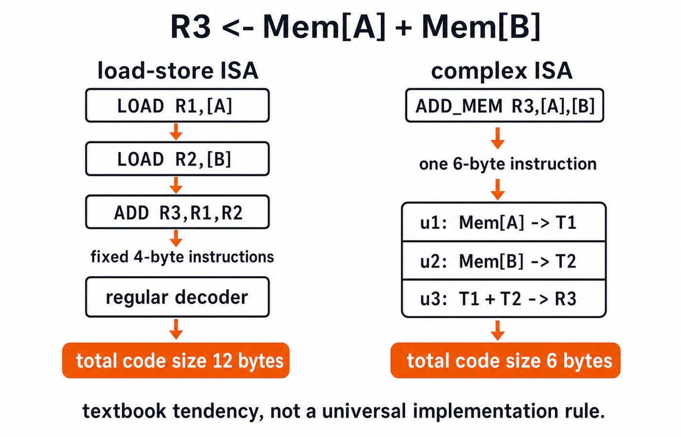
The complex instruction can be represented by these internal steps:
u1: Mem[A] -> T1u2: Mem[B] -> T2u3: T1 + T2 -> R3
The load-store version exposes three instructions that can be decoded directly. The complex version exposes one instruction whose internal sequence performs the same abstract work. A microinstruction does not always consume exactly one clock cycle, and not every CISC instruction is microcoded.
RISC vs CISC worked instruction example
Consider two hypothetical teaching ISAs, not ARM, RISC-V or x86. Both compute R3 <- Mem[A] + Mem[B].
In the load-store sequence, the first instruction copies Mem[A] into R1, the second copies Mem[B] into R2, and the third adds those registers into R3. The complex instruction names both memory operands at once. For these teaching ISAs, use the stated byte lengths as assumptions.
The load-store ISA uses:
LOAD R1,[A]LOAD R2,[B]ADD R3,R1,R2
At a fixed 4 bytes per instruction, its code size is:
3 x 4 bytes = 12 bytes
The complex ISA defines one instruction, ADD_MEM R3,[A],[B]. At its stated variable length, its code size is:
1 x 6 bytes = 6 bytes
Therefore, its encoding uses half the instruction bytes for this operation because 6 / 12 = 0.5. That conclusion concerns code size only. CPU time still depends on internal work, CPI, clock period and memory behaviour.
RISC vs CISC CPU-time worked example
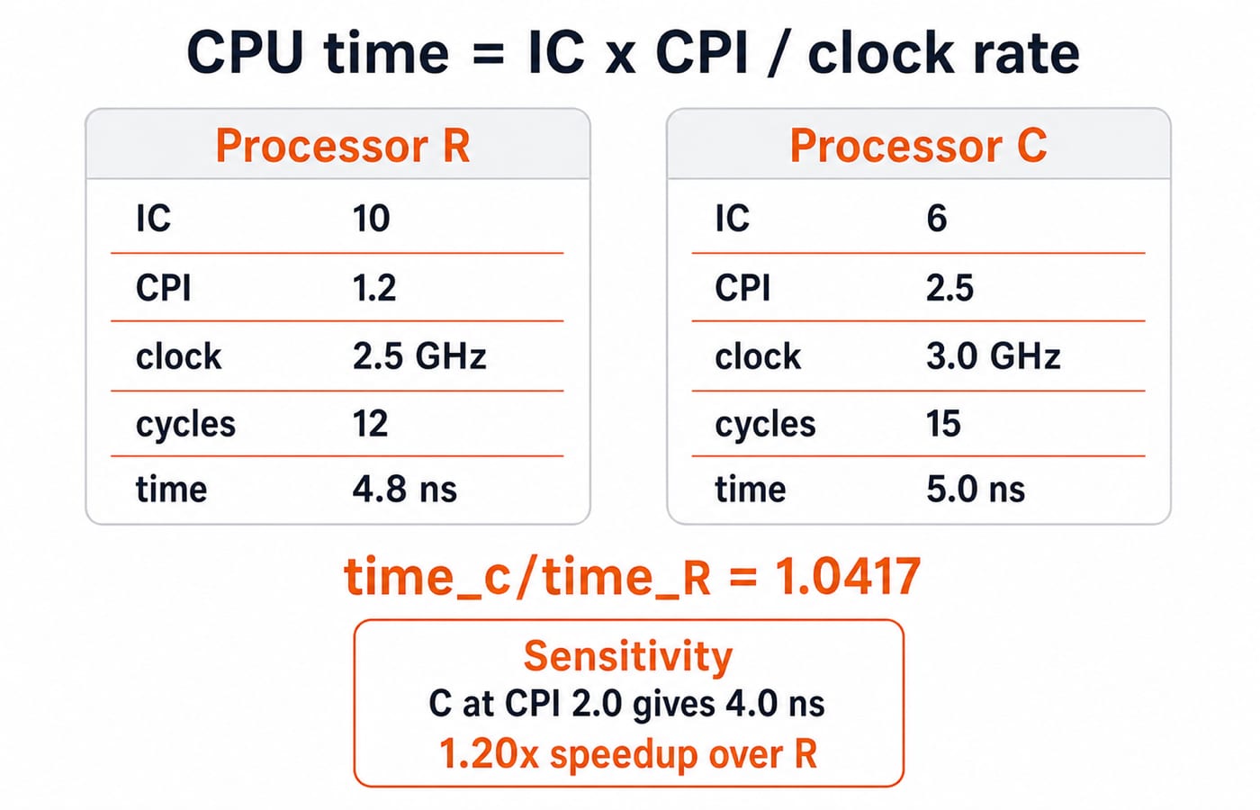
For one fixed workload, the valid comparison is:
CPU time = instruction count x average CPI / clock rate
Processor R executes 10 instructions at an average CPI of 1.2 and a 2.5 GHz clock.
Cycles =
10 x 1.2 = 12 cycles.Time =
12 / (2.5 x 10^9) seconds = 4.8 ns.
Processor C executes 6 instructions at an average CPI of 2.5 and a 3.0 GHz clock.
Cycles =
6 x 2.5 = 15 cycles.Time =
15 / (3.0 x 10^9) seconds = 5.0 ns.
For this workload, time_C / time_R = 5.0 / 4.8 = 1.0417. Processor R therefore has about a 1.042x speedup and uses 4% less execution time, despite executing more instructions. The given values cause the result, not the ISA labels.
Now reduce C's average CPI to 2.0 and leave everything else unchanged. Its time becomes 6 x 2.0 / 3.0 GHz = 4.0 ns. C is now 4.8 / 4.0 = 1.20x faster than R. The ranking reverses, proving that instruction count alone is insufficient.
RISC vs CISC traps: repair the shortcut
Shortcut | Why it fails | Correct test |
|---|---|---|
RISC always takes one cycle per instruction | CPI varies | Use average CPI |
CISC is always microprogrammed | Control styles can mix | Inspect the design |
Fixed length guarantees speed | Decode alone is not time | Calculate CPU time |
Fewer instructions mean lower time | C: 6 and 5.0 ns; R: 10 and 4.8 ns | Compare one workload |
Higher GHz always wins | IC and CPI matter | Use the formula |
Code size substitutes for execution time | 6 versus 12 bytes measures density | Check the requested measure |
At C's CPI of 2.0, time becomes 4.0 ns and the ranking reverses. Keep units on every line. Convert GHz to cycles per nanosecond once.
Ask: What is visible in the ISA? What happens internally? What are IC, CPI and clock rate for the same workload? Is the target density, cycles or elapsed time?
How exams test RISC vs CISC architecture
Recurring question forms include matching architectural features, judging statement sets with false absolutes, distinguishing hardwired and microprogrammed control, tracing micro-operations, comparing code size, and solving IC x CPI / clock rate numericals. These are common question forms, not a fixed paper pattern.
Recognise the requested quantity before calculating. A code-density prompt uses 12 bytes versus 6 bytes. A cycle prompt uses 12 cycles versus 15 cycles. A time prompt also needs 2.5 GHz versus 3.0 GHz. These comparisons cannot share one conclusion.
More than 20 questions on RISC vs CISC Architecture are available in the KnowledgeGate practice bank. Use the GATE Test Series to apply the method under timed conditions.
RISC vs CISC architecture: the short version
ISA style is not processor speed. Classic RISC tends towards regular load-store instructions, while classic CISC tends towards richer variable encodings. Performance must still be calculated for the stated workload: R takes 4.8 ns versus C's 5.0 ns, but C falls to 4.0 ns when its CPI changes.
For control-signal generation and microinstruction formats, the Control Unit Design in COA note owns the detailed treatment; here, control style matters only as one RISC-versus-CISC tendency. Next, connect regular instruction flow to the Pipelining in Computer Architecture Explained note.
Keep learning
Memory Chip Configuration: Chip Count, Address Lines and Two Worked Designs
Learn to separate depth expansion from width expansion, wire chip banks, derive address pins and check hexadecimal ranges with two complete examples.
Updated 25 Oct 20265 min readComputer Organization & Architecture
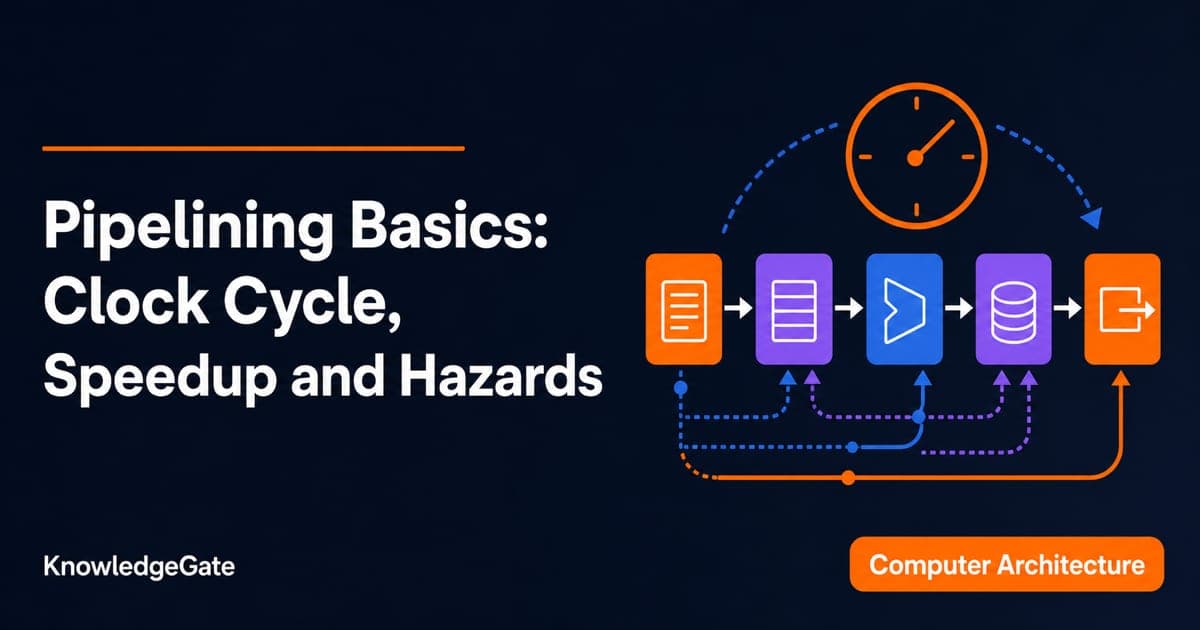
Pipelining Basics in Computer Architecture: Clock Cycle, Speedup and Hazard Worked Examples
Learn how to calculate a pipeline clock, fill and drain time, finite-batch speedup, latency, throughput, and the cost of a load-use stall.
Updated 23 Oct 20266 min readComputer Organization & Architecture

Data Manipulation Micro-Operations in COA: Arithmetic, Logic and Shift Operations Worked Step by Step
Learn a fixed-width method for tracing arithmetic, logic, and shift micro-operations. Every example tracks register values, result bits, carry, and overflow.
Updated 19 Oct 20265 min readComputer Organization & Architecture
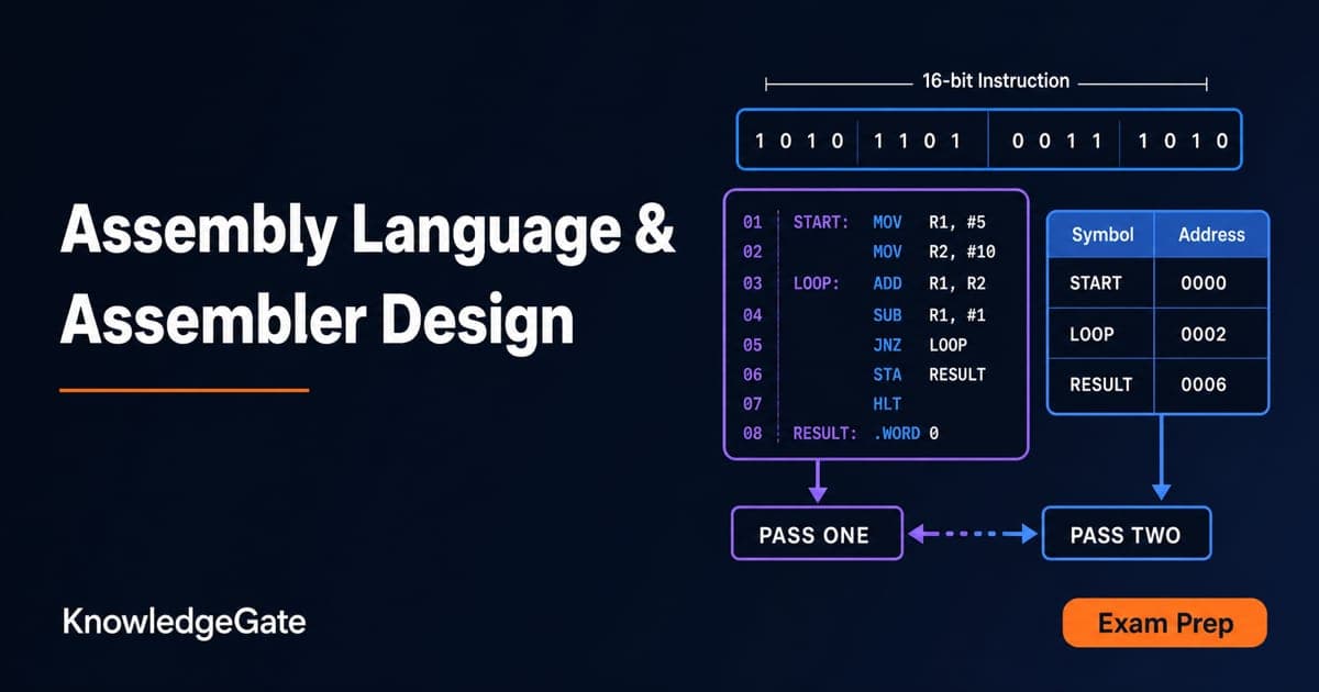
Assembly Language and Assembler Design: Two-Pass Translation with a Complete Worked Example
Follow a 16-bit Basic Computer program through pass one, pass two, hexadecimal encoding and execution, with every symbol, address and result shown.
Updated 15 Oct 20266 min readComputer Organization & Architecture